Module propagation_model

What is propagation model?

In this library propagation model is considered as one or a plenty of phenomenas acting in one network, e.g. Suspected-Infected model.

Purpose of PropagationModel module

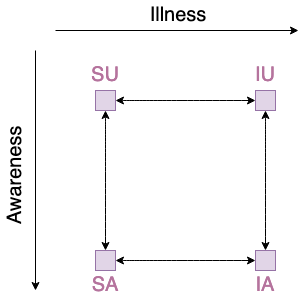
If experiment includes more than two phenomenas interacting with themselves, description of the propagation model becoming very complicated. E.g. model with 2 phenomenas with 2 local steps each:

• Suspected-Infected (phenomena Illness),

• Aware-Unaware (phenomena “Awareness”),

has 4 possible global states (i.e. for multiplex network each node has to be in one of those states):

• Suspected~Aware

• Suspected~Unaware,

• Infected~Aware,

• Infected~Unaware

and 8 possible transitions (i.e. possible ways for nodes in Multiplex network to change states):

• Suspected~Aware -> Suspected~Unaware,

• Suspected~Aware <- Suspected~Unaware,

• Infected~Aware -> Infected~Unaware,

• Infected~Aware <- Infected~Unaware,

• Suspected~Aware -> Infected~Aware,

• Suspected~Aware <- Infected~Aware,

• Suspected~Unaware -> Infected~Unaware,

• Suspected~Unaware <- Infected~Unaware.

This can be easily visualized by graph:

Note that with 3 phenomenas of respectively 2, 2, 3 local states we have 12 global states with (sic!) 48 possible transitions. This is so big value, that without computer assistance it is difficult to handle cases like this. Thus library contains module named propagation_model to define model in semi automatic way with no constrains coming from number od phenomenas and number of states. User defines names of phenomenas, local states and only these transitions which are relevant to the simulation.

Example of usage

Let’s define model with 3 phenomenas, 2 (layer_1, layer_2) with 2 local states each (A, B) and 1 (layer_3) with 3 local states (A, B, C). Then assign probabilities of transitions between certain states.

Define object of model propagation:

from network_diffusion import PropagationModel
model = PropagationModel()

Assign phenomenas and local states. Then compile it ad see results:

model.add('layer_1', ('A', 'B'))
model.add('layer_2', ('A', 'B'))
model.add('layer_3', ('A', 'B', 'C'))
model.compile()
model.describe()

============================================
model of propagation
--------------------------------------------
phenomenas and their states:
layer_1: ('A', 'B')
layer_2: ('A', 'B')
layer_3: ('A', 'B', 'C')
background_weight: 0.0
layer 'layer_1' transitions with nonzero probability:
layer 'layer_2' transitions with nonzero probability:
layer 'layer_3' transitions with nonzero probability:
============================================

Assign nonzero probabilities to the propagation model code:

model.set_transition('layer_1', (('layer_1.A', 'layer_2.A', 'layer_3.A'),
    ('layer_1.B', 'layer_2.A', 'layer_3.A')), 0.5)
model.describe()

============================================
model of propagation
--------------------------------------------
phenomenas and their states:
    layer_1: ('A', 'B')
    layer_2: ('A', 'B')
    layer_3: ('A', 'B', 'C')
    background_weight: 0.0
layer 'layer_1' transitions with nonzero probability:
    from A to B with probability 0.5 and constrains ['layer_2.A' 'layer_3.A']
layer 'layer_2' transitions with nonzero probability:
layer 'layer_3' transitions with nonzero probability:
============================================

Set random transitions and see all model:

model.set_transitions_in_random_edges([[0.2, 0.3, 0.4], [0.2], [0.3]])
model.describe()

============================================
model of propagation
--------------------------------------------
phenomenas and their states:
    layer_1: ('A', 'B')
    layer_2: ('A', 'B')
    layer_3: ('A', 'B', 'C')
    background_weight: 0.0
layer 'layer_1' transitions with nonzero probability:
    from A to B with probability 0.2 and constrains ['layer_2.A' 'layer_3.A']
    from B to A with probability 0.3 and constrains ['layer_2.B' 'layer_3.A']
    from A to B with probability 0.4 and constrains ['layer_2.B' 'layer_3.C']
layer 'layer_2' transitions with nonzero probability:
    from A to B with probability 0.2 and constrains ['layer_1.B' 'layer_3.B']
layer 'layer_3' transitions with nonzero probability:
    from C to B with probability 0.3 and constrains ['layer_1.B' 'layer_2.B']
============================================

Because of the propagation model is stored as a dictionary of networkx graphs, user is able to draw it, but as the model is bigger as the readability of visualisation is less:

import matplotlib.pyplot as plt
for n, l in model.graph.items():
    plt.title(n)
    nx.draw_networkx_nodes(l, pos=nx.circular_layout(l))
    nx.draw_networkx_edges(l, pos=nx.circular_layout(l))
    nx.draw_networkx_edge_labels(l, pos=nx.circular_layout(l))
    nx.draw_networkx_labels(l, pos=nx.circular_layout(l))
    plt.show()